This is a recap post for a whitepaper I released while mentoring FRC team 88. I introduced LIDAR-based localization with ROS into their ecosystem. It provided localization for their autonomous programs and saw the world stage in Houston Texas in 2022.

Links to the original posts:

• https://www.chiefdelphi.com/t/using-ros-for-inspiration-in-frc/411561
• https://www.chiefdelphi.com/t/rosnetworktablesbridge-a-better-way-to-connect-wpilib-java-and-ros/437914

---

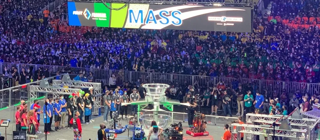
For the 2022 season, FRC team 88 TJ² implemented LIDAR based localization using ROS on our robot. This tool unlocked the ability to localize our robot on the field even with heavy defensive maneuvers by the opponents. Above you can see qualification match 35 at the 2022 FIRST world championship (Galileo division) with a twist! In the bottom screen, you can see ROS’ recording of the match. The orange box represents the robot’s estimated position (the bottom video is roughly overlaid on the top video as well). This is not a simulation run after the match, but a recording of localization that was running live on the robot.

This demo has been part of an effort to showcase tools that real production and development robots use recontextualized for FIRST. The ultimate goal is to make these tools easily accessible to all FIRST teams. Hopefully, this will inspire more students to pursue a career in robotics and prepare them for the problems they will solve. In this paper, I will detail why ROS is not just a gimmick in FIRST, but an advanced tool that can augment the performance of any robot. I will also outline the exciting potential future for ROS in FRC.

ROS is not an easy tool to pick up, but shows great potential. We want to make these tools available to other FIRST teams as well as expand its capabilities and performance. If this kind of work sounds interesting to you, please reach out on this Chief Delphi post.

Background

But what exactly is ROS and why are we so excited about it? The ROS website explains its own background pretty well, but for us, it’s a tool that connects advanced robotics algorithms to robot specific hardware using standardized messaging protocols. An analogy I like to use is getting the latest news. Imagine you want to stay informed about local events in your town. You could go to every neighbor, church, restaurant, or government building and ask what’s happening that week. This is quite laborious and chances are there’s already a town newspaper that collects this information. The sensible thing to do would be to subscribe to the newspaper to get updates.

In our case, ROS is the local newspaper and developing your own robotics stack is asking everyone yourself. A lot of institutions and individuals have already written code for the ROS ecosystem and all we need to do as developers is install and configure it. I like to use the newsstand analogy specifically because ROS utilizes the subscriber-publisher model of passing data around. A node will publish a message on a topic, and any nodes subscribed to that topic will receive that message. What this means is if I write a magical algorithm that subscribes to camera images and returns your exact GPS coordinate, any camera that publishes that message type can plug into this algorithm. Plus, any code that utilizes GPS coordinates can immediately use the output of my algorithm with no modifications.

Team 88’s use case

Shooting cargo with LIDAR localization

We use LIDAR-based localization to get our location on the 2022 Rapid React field. The magical algorithm of choice is AMCL. It subscribes to LIDAR and wheel odometry data and returns a corrected position relative to the origin of the mapped area. We selected LIDAR units that come with a ROS driver (the RPLIDAR A2M8) and formatted our wheel odometry into the ROS odometry message.

This unlocks the ability to shoot cargo from anywhere on the field, even when the retro-reflective targets on the goal are blocked. In addition, it means shooting while moving becomes a trivial trigonometry problem. Looking back at the GIF at the beginning of this document, you can see a red arrow darting around the center of the bottom image. This is the selected target of our robot. We know where we are and that the target doesn’t move, so we simply select the center coordinate as the target. We collected time-of-flight for our shots at increasing distances to create a distance-to-time table. We multiply those times by our current robot’s velocity and subtract this distance from the current target to get our compensated shot. If our velocity is changing (accelerating or decelerating) we decrease the probability that the shot will go in. If the probability is above a certain value, it will shoot automatically.

There were several key challenges we had to solve to get this system to work at worlds. The first was maximizing LIDAR field-of-view and range. If the LIDARs can see more, AMCL has more opportunities to lock onto the true position. With one LIDAR unit on our 2020 robot, our FOV was 120 degrees. We found this was inadequate for localization. The system would sometimes never converge on its actual position. On this year’s robot, we get ~190 degrees with one LIDAR. This is fine, but there are many instances where the LIDAR is blinded when close to a wall or blocked by a robot. We added two LIDARs to increase the range to 300 degrees. This ensures we have at least one wall in view at all times. Ideally we would have put the two LIDARs on opposite corners for the full 360, but our intake geometry prohibited this.

The next challenge was dealing with clear polycarbonate. There was an obvious concern that shooting a laser at clear material would not work. Pointing the LIDARs at the metal field barrier beams was infeasible because the target is so small. The robot tips a lot and tolerances between fields can vary. It would more likely catch the stands or judges table. So we had to mount the LIDARs below the field barrier height.

Surprisingly, the LIDARs we selected can see the clear polycarbonate as a solid wall, but only from a reduced set of angles.

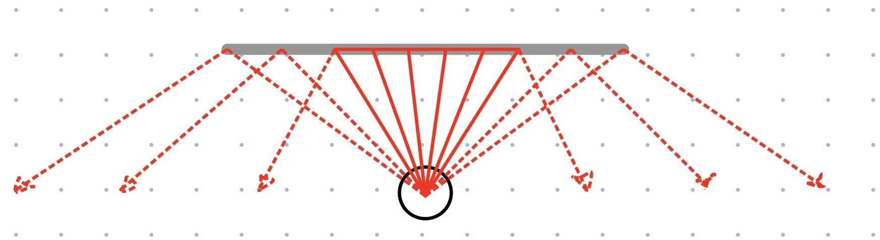
Past a certain angle, not enough light is reflecting back to the LIDAR unit for it to register a distance measurement. Despite this reduction in usable sensor data, AMCL is still able to work.

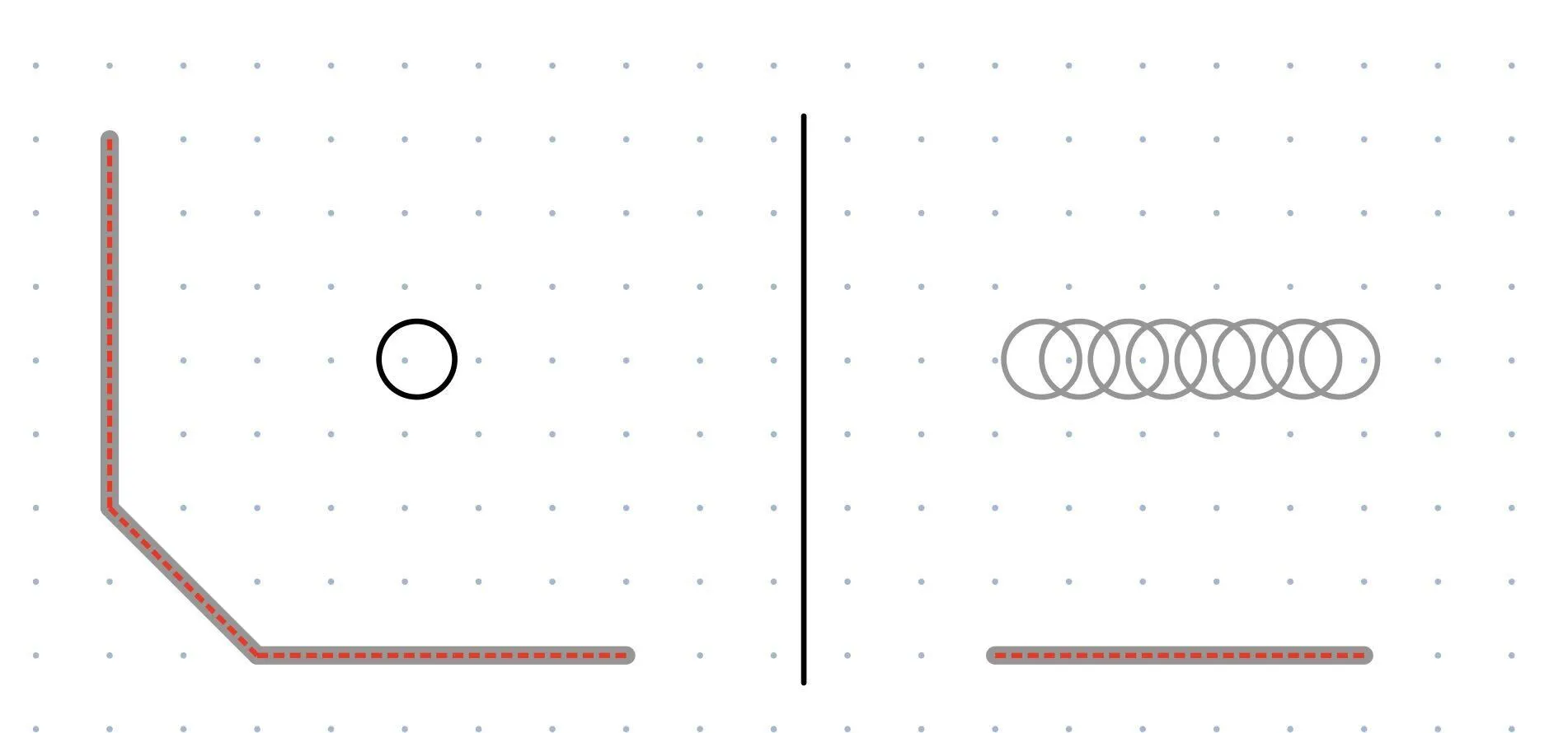
A key factor of getting AMCL to converge quickly is having orthogonal walls. In the left image, the LIDAR is aligned with the vertical and horizontal walls. In 2 dimensions, there is nowhere else this robot could possibly be. In the right image, the LIDAR only sees a horizontal wall. The robot could be anywhere along that wall and produce the same measurement, so its position is more uncertain. For these reasons, we selected LIDAR settings that would give us the longest range (RPLIDAR’s “Boost” mode) and mounted them in a way that would maximize FOV.

Another wrinkle was we had to teardown our field setup almost everyday. Re-drawing the map by hand for every session is tedious and wastes precious time. Here’s a map of the room we tested in:

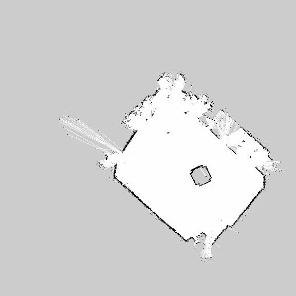
And this is the map we used for the Rapid React field:

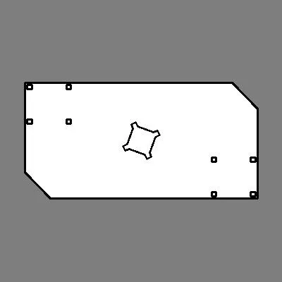
Our robot has the ability to generate its own maps using a technique called SLAM (Simultaneous Localization And Mapping). Essentially, it can merge together LIDAR scans as the robot moves about the room and build a complete map of the area. We can then freeze this map and use it with AMCL for localization. The ROS tool for this is called gmapping. So, while it was annoying to remap the field every session, it was much faster than measuring the furniture locations and drawing a new map by hand.

After we had proved this setup for localization and shooting worked on the practice field, we needed to transfer these settings to the real field. To generate the field map, we selected points from CAD that line up with what the LIDARs see and drew an image. Because each field is the same (or same enough), no on-field calibration is required. The same AMCL settings work on the practice field and the real field. AMCL requires that you give it an estimate of starting location otherwise it will take a few minutes to automatically converge as it tries every position on the map. We transferred these set starting locations from the practice map to the real map and it was good to go.

The last challenge was reducing system latency. These issues mostly came from the roboRIO and Jetson not having enough CPU bandwidth. We resolved this by decimating the amount of data we push to SmartDashboard, reducing redundant calculations and sensor polling, and reduced the number of positions AMCL checks every iteration. We found if odometry is not given to AMCL for at least 0.15 seconds and the robot is moving fast, it’s possible the system will become lost and not converge until just before the match is over. In the end, we got NetworkTables to provide odometry with ~0.05 seconds of latency on average.

Automatically picking up cargo

We implemented auto cargo pursuit and shooting during autonomous mode. If you’re not familiar with the Rapid React strategies, there were essentially 3 roles for the autonomous period this year: 5 ball, 2 ball, and 1 ball autos.

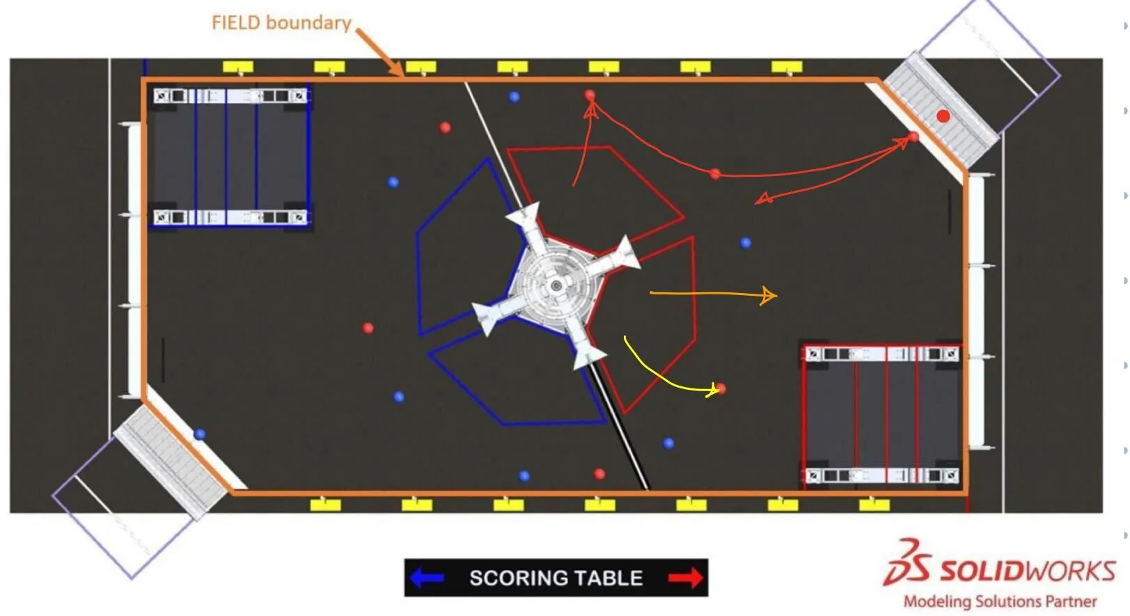
• “5 ball auto” is the red path. Shoot the preloaded cargo. Drive into the 1st and 2nd ball and shoot. Drive to the farthest 3rd ball. Pick up the last ball which is rolled in by the human player. Drive back and shoot.
• “2 ball auto” is the yellow path. Shoot the preloaded cargo. Drive backwards and pick up the cargo and shoot.
• “1 ball auto” is the orange path. Back up and shoot the preloaded cargo.

These are traditionally done with pre-computed trajectories. The alliance collaborates before the match to ensure no collisions occur. It’s impossible to predict where the cargo will be after it bounces out of the hub, so you can only rely on the preplaced cargo locations. What ends up happening is the “5 ball auto” robot spends all 15 seconds running its route and the other two twiddle their thumbs for 5-10 seconds after they’re done. Our objective with cargo pursuit was to capture cargo that falls out of the hub after the 1 ball or 2 ball auto finish.

To do this, we need a way of identifying where the cargo is. Then, the robot drives to the cargo and ensures we don’t hit teammates or field elements along the way. I’ve seen a few teams try the traditional computer vision approach. This works great for this year’s game because the game pieces have a high contrast to other objects. This approach involves filtering for either red or blue pixels in an image and applying a blob detector.

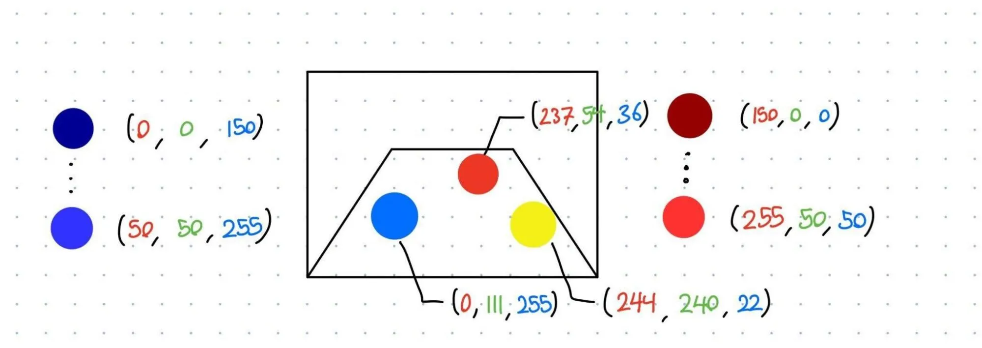
Imagine you have a red, blue, and yellow ball in your camera’s view. In order to find them, you can apply thresholds to the red, green, and blue channels in the image. In this case, the red and blue balls pass our selected threshold because all 3 channels are within the bounds. The yellow ball’s red and blue channels are within our threshold, however, the green does not, so it’s ignored. The output of this threshold is a black and white image with a 0 or 1 in each pixel. 1 for within the threshold, 0 for not. A blob detector simply groups “1” pixels that are adjacent to each other and returns a set of coordinates.

This pipeline is highly dependent on ambient conditions and not robust to situations where two similar objects are close to each other. If it’s a particularly bright or dark arena, you’ll likely have to adjust your thresholding values for what counts as “red” or “blue”. The Limelight has tools that solve the exact same problems.

We did not use this approach. We opted for the nuclear solution. What if we could create a detector that worked on any FRC game object on any field without on-site calibration? YOLOv5 was the obvious choice for this. This library implements an object detection algorithm, a type of neural network. This neural network specializes in drawing boxes around predefined objects. We provided YOLOv5 with 1726 images of red and blue cargo. It generated a pipeline that, when fed an image it has never seen before, will return a list of coordinates defining where the objects are in the image. At first, we tried MobileNet V2 via jetson-interference’s detectnet but found its performance to be vastly inferior. MobileNet V2 would frequently identify blank space as cargo or not identify actual cargo despite ample training data for other datasets we tried. I triple checked for errors like reversed color channels (interpreting blue as red and vice versa) and mislabeled training data.

YOLOv5’s success rate is far superior and processes images just as fast on the Jetson. Here’s YOLOv5 running on our robot during a match:

Red and blue cargo is correctly identified. A concern was opponent robot bumpers being mistaken for cargo. As seen in the video, no bumpers were mistaken for cargo. You may notice that we’re drawing the cargo’s position in 3D. There’s one more step to our pipeline and that involves our depth camera.

Drawing a box in an image doesn’t resolve its 3D position. The object could be very large and far away, or very small and close up. We can roughly gauge distance since we know the size of the object, but that’s not what we decided to do. We utilize the depth module on our camera, the RealSense L515. It has the ability to generate a depth image where every pixel is a distance from the camera in millimeters.

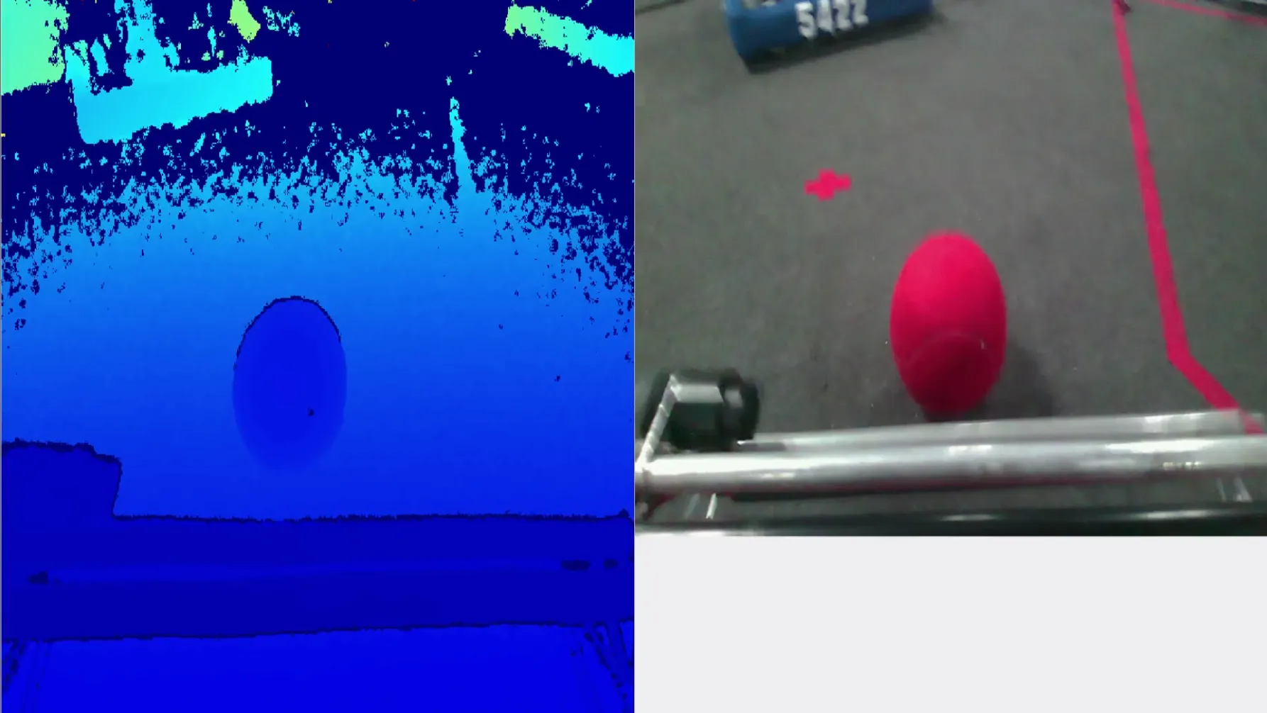
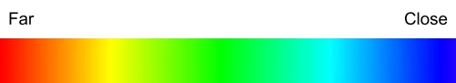
On the left is the depth camera. On the right is the color camera. Blue colors indicate pixels that are close to the camera. Here’s a rough legend describing the coloring:

After YOLOv5 has identified an object, we simply take the average pixel value in that region of the depth image and use that as the object’s distance from the camera. This strategy worked because the cargo is a sphere, so we don’t care about the orientation of the object. If we care about the object’s orientation in next year’s game, we’ll need a more clever strategy for figuring out which direction the object is pointed.

Now that we have the object’s position, we need to tell the robot to drive to it. ROS has tools for guiding robots to goals. Here’s a link to a demo video of our test bot doing that. This tool is called move_base. Here’s a great tuning guide if you’re curious about using it. Unfortunately ROS 1 doesn’t have an easy way of commanding goals that move or update rapidly. Two of move_base’s states are the “planning” and “controlling” states. In the planning state, it has received a goal and is generating a path to it. Once a path is generated, it enters the controlling state where a local planner publishes velocity commands that get the robot to follow the path. If we continuously send goals to move_base, it will constantly switch to the planning state and never run the controlling state. A fix for this is shortening the amount of time the planning state takes by selecting a simpler path planner. move_base has the ability to swap out what type of path planner you use. The default is global_planner. It generates paths that avoid obstacles according to your map as well as unexpected obstacles that are detected by your sensors. On our hardware, it’s happiest when running at 1 Hz. This update rate is too slow for pursuing moving cargo. carrot_planner is much simpler. It just picks the nearest unobstructed point between the robot and goal and tells the robot to go there. We can run this planner at 10 Hz or more.

Here’s a demo of that code:
Successful attempt
Unsuccessful attempt

The problem we encountered was the cargo would leave the frame of the image too quickly and the planner would stop. We either needed to increase our field of view or prioritize keeping the cargo in the frame. It’s possible to write your own local planners for move_base. We could modify an existing planner like dwa_local_planner to prioritize pointing the robot at the goal instead of getting it onto the global path. For lack of time however, we employed a simple PID controller. If the cargo is to the left of the robot, it turns left. If the cargo is to the right of the robot, it turns right. Drive forwards until the cargo is within a certain distance. We only ran this mode a couple of times during the season since we didn’t run our 2 ball auto very often. This video shows this code running successfully during NE championships. Watch our robot (88) in the bottom right. We had just finished our 2 ball auto. Cargo slowly rolled into frame just in time for the robot to pick it up. Unfortunately by the time the robot saw the cargo and picked it up, the autonomous period was over.

There are many issues with this setup that make it difficult to justify use during teleop or even most autonomous modes. The main issues I see are the poor FOV from the RealSense camera, slow reacting controllers and path planners, and lag from the camera and neural net. From testing, we found it takes around 0.1 seconds for the image to propagate from the camera to the start of the neural net pipeline. I’ve searched around for ways to improve this. I suspect it has to do with synchronizing the depth and color images. You don’t want images taken too far apart otherwise you’ll get incorrect distance measurements. However, the algorithm that syncs them might be taking too long. The neural net runs at around 20 to 30 FPS. This means it adds 0.05 to 0.033 seconds of lag for every image. Unfortunately I can’t do much to speed this up. We’re using the lightest model YOLOv5 offers (yolov5n) and the most powerful GPU an FRC budget will allow.

Poor FOV could be fixed by adding more RealSense cameras of course, but this will overrun our CPU bandwidth. We could also add regular cameras running at a lower resolution. If we add a fisheye lens, we could cover much more ground. These cameras would just tell the robot which direction to rotate while the RealSense camera provides a more accurate position when the object is in view. We could also add a depth camera to the driver station and send object locations to the robot.

There’s certainly a lot of improvements to be made with the path planning. Writing a custom local planner is an option, but not having a smart global planner is detrimental. This might be a case for switching to ROS 2, which has a package called Nav2. This package has demos for dynamic object following.

Unexplored use cases

There’s so much potential with this software. My dream is to one day deploy a fully autonomous, competitive FRC robot. There’s a lot of barriers that prevent this from happening in FRC today, however there is a fair amount of semi-autonomous functionality that is possible. For this year’s game, we could create a dashboard that displays the location of all cargo the robot sees on the field and highlights larger clusters. Often drivers would miss cargo because it had rolled into their blind spots. For semi-auto routines, the robot could do light course correction to the cargo while avoiding other obstacles. 2020’s game had a see-saw hang bar that, when balanced, would award the team extra points. We can use the depth camera to see what angle the bar is and automatically position the robot so that the bar becomes balanced. Or at the very least, position climbing hooks so they only go as high as they need to and save precious seconds. Some games require more precise placement of objects like 2017’s Steamworks. Using the depth camera, precise pick and place routines become possible. A neural net can not only recognize object locations but where to place them as well. A motion planner can figure out the best path between the held object and the destination and execute the routine automatically. No more fiddling with joystick controls under stressful competition situations.

There are a few issues we need to overcome in order to make this a reality. Besides the issues I mentioned like camera FOV and lack of moving goal support from move_base, CPU usage is starting to become a problem. We find when using teb_local_planner, the system will frequently lock up and stop sending velocity commands for a split second. This causes the robot to send a full stop command as it realizes it has veered too far off course.

Here’s some stats on our CPU usage on the Jetson Xavier NX while the robot is idling:

Process name	Description	CPU usage (our Jetson has 6 cores, so full is 600%)
realsense2_camera_manager	Driver that interfaces with the camera	150%
tj2_yolo	YOLOv5 node	130%
tj2_depth_converter	smoothes out depth image	21%
pointcloud_to_laserscan_node	Converts camera output to single scan	20%
tj2_pursuit	object tracking PID controller	15%
tj2_waypoints	keeps track of waypoints on the map and runs the guidance state machine	15%
camera_post_processing_manager	aligns the depth to the color image	12%
amcl	Laser localization	5%

Our total idle CPU usage is 75% (out of 100%).

Here the processes that differ significantly while moving:

Process name	Description	CPU usage (our Jetson has 6 cores, so full is 600%)
move_base	Navigation and path planning	60%
amcl	Laser localization	28%

Our CPU usage while the robot is path planning is 90% (out of 100%).
Without the camera and neural net, our robot’s CPU usage while path planning is 23%.

So while navigation does take a significant amount of CPU, over half of our computing time is spent on handling the camera and neural net. I don’t know exactly what processing is done on the RealSense camera and what’s done on the Jetson, but I think it’s a bit crazy that a core and half is used just to process the camera’s data. This doesn’t include the extra stuff like shifting the depth image to line up with the color image or creating a point cloud.

We’ll need to switch to a different camera anyway since Intel is retiring this line of cameras. So, I’ve done a test with the ZED camera from Stereolabs and the CPU usage is significantly better. The FOV is wider and it appears the depth precision is adequate. In addition, using a more CPU efficient color-depth synchronization algorithm cuts tj2_yolo’s CPU down by half.

Process name	Description	CPU usage (our Jetson has 6 cores, so full is 600%)
tj2_yolo	YOLOv5 node	75%
zed_wrapper_node	ZED camera manager	25%

Now, idle CPU is 40%.

Unfortunately, the quality of the depth image is not as good. Details do not show up as well when compared with the L515. It remains to be seen whether this is an issue or not.

The future with ROS

ROS is a tool that will lead to more interesting games and more accurately prepare students for the future of robotics and engineering. It’s used by companies and academia for prototypes and final production. From personal experience, I’ve worked with teams at Amazon Robotics and CMU robotics labs that use it for prototyping. If students learn this tool, they will have skills directly translatable to future careers. Even if ROS is not the final tool of choice, production robots are 100% autonomous. There are little to no robots operated by joystick. By allowing nonresearchers to use these algorithms, ROS is offering a chance to study deeper into these fields.

I’m excited about what the distant future looks like with these tools in hand. What kinds of games would we be playing if everyone had fully autonomous robots? Maybe robots on the same alliance would communicate where they see game objects for a more complete view of the field. FIRST might see an opportunity to make games that require more nuanced perception of the field, like how objects are placed and oriented, tight maneuvers that are difficult to pull off from the driver station, setting the score multiplier based on a set of lights or field elements the robot needs to read. It may be viable to employ countermeasures to confuse the opponent, like blocking the most optimal path so the robot has to go around or confusing their localization by blocking their sensor view. The best localization system would be an overhead camera that wirelessly transmits the robot’s location. FIRST could add a “Zebra”-like camera system to the Field Management System (See: Zebra MotionWorks, scroll down for match playback).

Next steps

One point I haven’t talked about in this paper is the challenge of learning ROS. I’ve detailed how TJ² put together their system in this wiki. I would say understanding ROS alone is very easy. The problem is there’s a lot of prerequisites before one can actually make it useful. Some of these include:

• Linux command line and file system
• SSH and SFTP
• An understanding of C++ build systems
• Resolving project dependencies
• C++ programming
• Python programming
• systemd
• Data flow and management via NetworkTables
• Basic computer vision pipelines via OpenCV
• Particle filters
• Coordinate transforms and linear algebra

I’m sure I missed several required concepts on this list. There needs to be a scalable way of transferring this work. That’s where I need your help. For the use case of FRC, I’d say most of these prerequisites can be sidestepped with a collection of tools precisely tuned for FRC. Most of the headache of working with ROS is actually setting it up and running it. That will be the biggest hurdle in getting this system out to other teams. If you have experience deploying these kinds of systems at scale, please reach out. I’d love to learn more about Docker or whatever tool we decide to pick. The tools ROS provides for setting up and debugging the robot work for me, but less experienced teams may find it very difficult and non-intuitive. I certainly did when I started using ROS. I’d like to develop more FRC tailored tools that ease the pain of deploying this system. If this sounds at all interesting, please reach out on the Chief Delphi post and we’ll get in touch.

All of the issues encountered and steps taken to get this to work are the same challenges robotics engineers face. System integration is an essential part of robotics as there are many complex systems talking to each other. The techniques ROS uses to achieve autonomy in FRC are the same or similar to ones used for production robots. Creating more interesting games will increase audience engagement. Implementing these cool systems will inspire more participation from mentors and students. I hope other teams will join me in creating a system that’s usable for everyone so that we might bring these incredible tools to all aspiring engineers.

Links

Main github page: https://github.com/frc-88/tj2_ros
Branch of code that ran at worlds: https://github.com/frc-88/tj2_ros/tree/ship/2022-robot
Wiki page: https://github.com/frc-88/tj2_ros/wiki
Chief Delphi post: https://www.chiefdelphi.com/t/using-ros-for-inspiration-in-frc/411561

~Benjamin Warwick, 2022, Team 88 TJ²